Just in order to get some more familiarity with joint PDFs, let us look at independent normals.
Actually, this is an important example because noise is often modeled by normal random variables, and noise terms that show up at different parts of a system, or at different times, are often assumed to be independent.
Suppose that we have two standard normal random variables, X and Y, with zero means and unit variances.
If their independent, their joint PDF is the product of the marginal PDFs and takes this form.
This is just the PDF of a standard normal X and the PDF of a standard normal Y and we multiply them.
If we are to plot this joint PDF we obtain this figure.
It looks like a bell which is centered at the origin– at the point with coordinates zero, zero.
One way to think about what is going on here is to rewrite this expression as 1 over 2pi, and then the exponential of minus 1/2 x squared plus y squared.
If we look at the unit circle in xy space, which is the set of points at which x squared plus y squared is equal to 1, then, on that circle, the PDF takes a constant value because this quantity is constant on that circle.
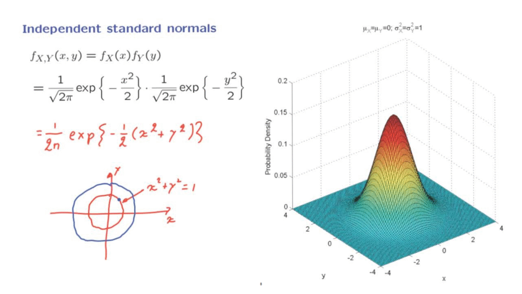
And the same is true for any other circle.
On any circle the PDF takes a constant value, of course, a different constant.
So the circles centered at the origin are the so-called contours of the joint PDF.
On each contour the joint PDF is a constant.
Let us now generalize.
Consider two independent normal random variables, but with general means mu x and mu y, and variances sigma x squared and sigma y squared.
The joint is, again, the product of the marginal PDFs and, therefore, takes this form.
This looks intimidating but, in fact, it is pretty simple.
This part is just a normalizing constant.
It is the constant that’s needed so that the joint PDF integrates to 1.
What we have here is the negative exponential of a quadratic function of x and y.
Let us plot the contours of this quadratic.
Remember that contour is the set of points where the quadratic takes a constant value.
And by consequence, the joint PDF also takes a constant value.
If you have set this quadratic to a constant, what you have is the equation that describes an ellipse.
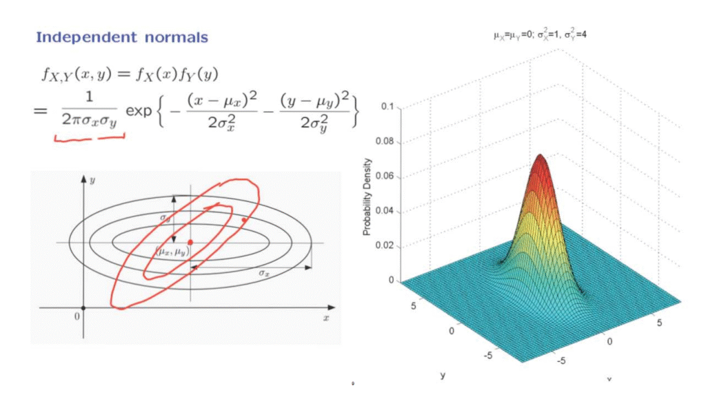
And it is an ellipse whose principal axes run along the x and y directions, and those ellipses are all centered at this particular point, mu x, mu y.
The joint PDF is largest when the exponent is equal to zero.
And this happens when x is equal to mu x, and y is equal to mu y.
That is, right at the center of the ellipse.
That’s where the joint PDF is largest.
As you move to ellipses that are further out on this outer ellipse, this expression is a constant.
It’s the exponential of the negative of some positive numbers.
So you get a smaller value for the joint PDF.
If you move to a further ellipse further out, then again, the joint PDF will be a constant, but it’s going to be a smaller constant.
Now, for the case of standard normals, the joint PDF was circularly symmetric.
The contours were actually circles, instead of ellipses.
But this is not the case in general.
For example, suppose that the variance of Y is bigger than the variance of X.
Then you get a shape as the one shown in this figure.
Since the variance of Y is larger, we expect Y to take values over a bigger range, and to be larger typically than the values of X.
And so the bell shape that we have for the joint PDF is stretched in the y direction.
It extends further out in the y direction than it does in the x direction.
To conclude, the joint PDF of two independent normals has the shape of a bell.
The center of the bell is determined by the means.
Furthermore, the bell is stretched in the x and y directions by an amount that is determined by the variances of x and y.
However, the stretching is always along the coordinate axes.
If you wanted a bell that stretches in some diagonal direction, or if you have contours that are ellipses but with some different kinds of axes, then you will have dependence between the two random variables.
In that case, we will be dealing with a so-called bivariate normal distribution, but we will not pursue this any further at this point.