The definition of the conditional PDF is very simple.
It is just this formula, which is analogous to the one for the discrete case.
In all respects– mathematical and intuitive– it is very similar to the conditional PMF.
Even so, developing a solid grasp of this concept does take some further thinking, so we will now make some observations that should be helpful in this respect.
The first and obvious observation is that the conditional PDF is non-negative.
It’s defined when the denominator is positive, the numerator is a non-negative quantity, so it’s always a non-negative quantity.
A more interesting observation is that for any given value of little y, the conditional PDF looks like a slice of the joint PDF.
Indeed, if you fix the value of little y, then the denominator in this definition is a constant, and we have a function that varies with x the same way that the joint PDF varies with x.
Pictorially, let us consider this particular joint PDF, and let this be the x-axis and let that be the y-axis.
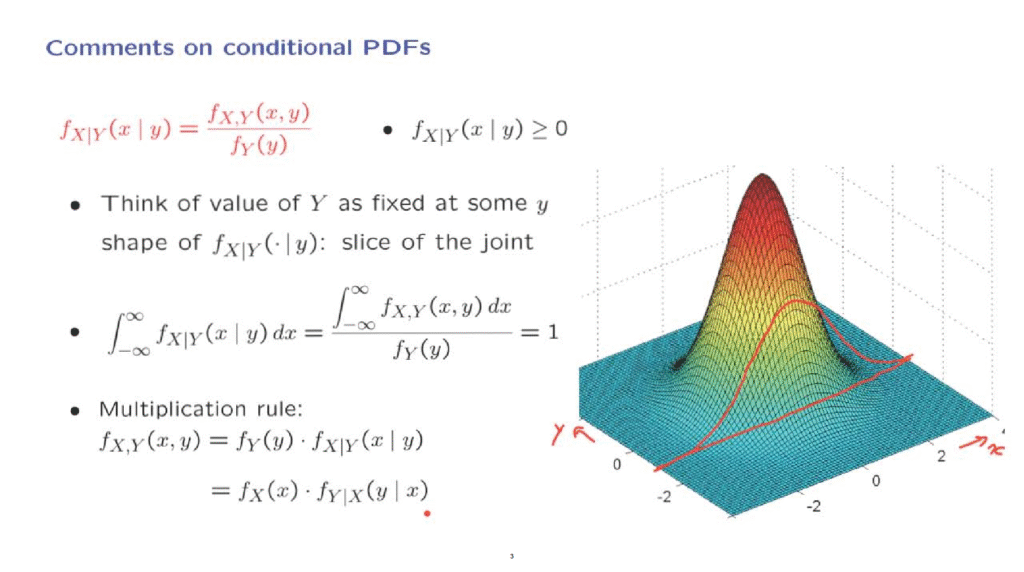
If we fix a certain value of y, if we condition on Y having taken this particular value so that our universe is now this particular line, on that universe the value of the denominator in this definition is a constant, and the conditional PDF is going to vary according to the height of the joint on that particular conditional universe.
So the height of the joint, if we trace it, is one of those curves up here, and [then] goes down.
So it is really a slice taken out of the joint PDF.
If we condition on a different y, we get a different slice of the joint PDF, and so on.
Actually, the conditional is not exactly the same as the slice.
We also have this term on the denominator that serves as a scaling factor.
It turns out that this scaling factor is exactly what we need for the conditional PDF, given a specific value of little y, to integrate to 1.
Indeed, if we fix little y and take the integral over all x’s, using the definition, and because this term is a constant and does not involve x, we only need to integrate the numerator.
And we recognize that the numerator corresponds to our earlier formula for the marginal distribution– the marginal PDF of Y.
From the joint, this is how we recover the marginal PDF of Y.
So the numerator turns out to be the same as the denominator, and so we get a ratio 1.
Therefore, the conditional PDF for a given value of the random variable Y behaves in all respects like an ordinary PDF.
It is non-negative and it integrates to 1.
A last observation is that we can take this definition and move the denominator to the other side to obtain this formula, which has the familiar form of the multiplication rule.
The probability of two events happening is the probability of the first times the probability of the second given the first, except that here we’re not really dealing with probabilities, we’re dealing with densities.
By symmetry, a similar formula must also be true when we interchange the roles of X and Y.
So, algebraically, everything is similar to what we have seen for the case of discrete random variables.
It’s the same form of the multiplication rule, although the interpretation is a bit different because densities are not probabilities.