We now look at an example similar to the previous one, in which we have again two scenarios, but in which we have both discrete and continuous random variables involved.
You have $1 and the opportunity to play in the lottery.
With probability 1/2, you do nothing and you’re left with the dollar that you started with.
With probability 1/2, you decide to play the lottery.
And in that case, you get back an amount of money which is random and uniformly distributed between zero and two.
Is the random variable, X, discrete? The answer is no, because it takes values on a continuous range.
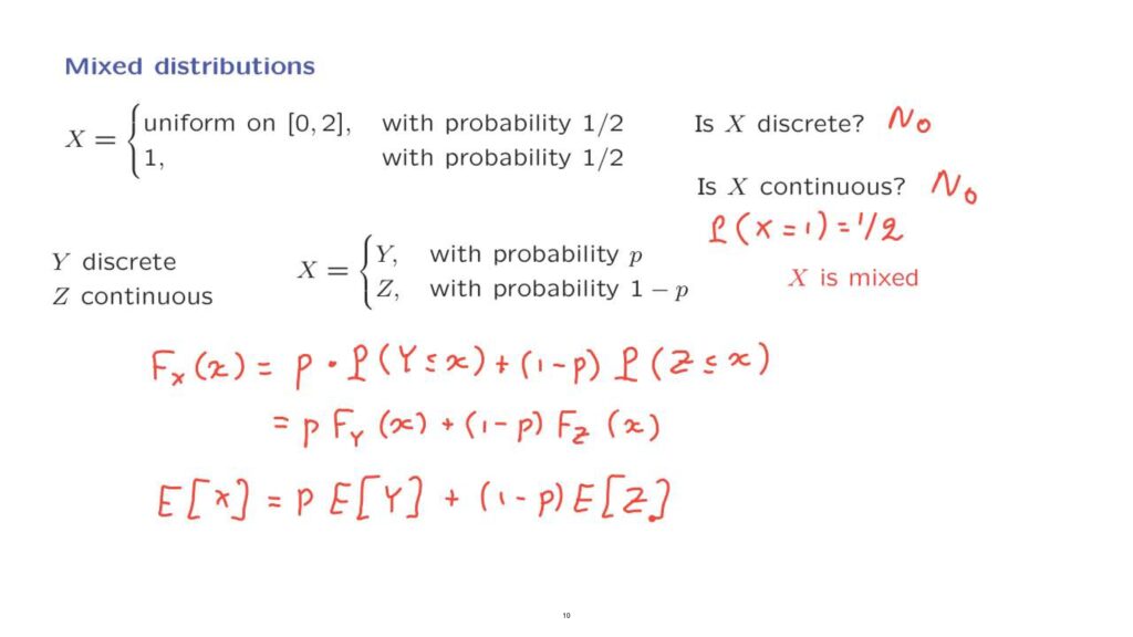
Is the random variable, X, continuous? The answer is no, because the probability that X takes the value of exactly one is equal to 1/2.
Even though X takes values in a continuous range, this is not enough to make it a continuous random variable.
We defined continuous random variables to be those that can be described by a PDF.
And you have seen it in such a case, any individual point should have zero probability.
But this is not the case here, and so X is not continuous.
We call X a mixed random variable.
More generally, we can have a situation where the random variable X with some probability is the same as a particular discrete random variable, and with some other probability it is equal to some other continuous random variable.
Such a random variable, X, does not have a PMF because it is not discrete.
Also, it does not have a PDF because it is not continuous.
How do we describe such a random variable? Well, we can describe it in terms of a cumulative distribution function.
CDFs are always well defined for all kinds of random variables.
We have two scenarios, and so we can use the Total Probability Theorem and write that the CDF is equal to the probability of the first scenario, which is p, times the probability that the random variable Y is less than or equal to x.
This is a conditional model under the first scenario.
And with some probability, we have the second scenario.
And under that scenario, X will take a value less than little x, if and only if our random variable Z will take a value less than little x.
Or in CDF notation, this is p times the CDF of the random variable Y evaluated at this particular x plus another weighted term involving the CDF of the random variable Z.
We can also define the expected value of X in a way that is consistent with the Total Expectation Theorem, namely define the expected value of X to be the probability of the first scenario, in which case X is discrete times the expected value of the associated discrete random variable, plus the probability of the second scenario, under which X is continuous, times the expected value of the associated continuous random variable.
Going back to our original example, we have two scenarios, the scenarios that we can call A1 and A2.
Under the first scenario, we have a uniform PDF, and the corresponding CDF is as follows.
It’s flat until zero, then it rises linearly.
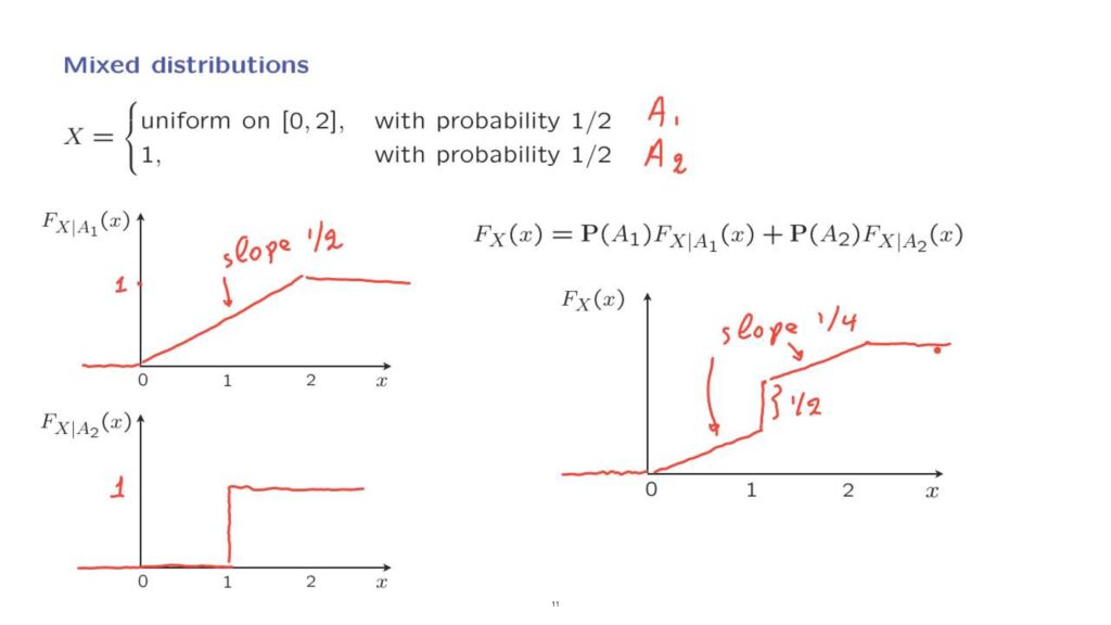
And then it stays flat, and the value here is equal to one.
So the slope here is 1/2.
So the slope is equal to the corresponding PDF.
Under the second scenario, we have a discrete, actually a constant random variable.
And so the CDF is flat at zero until this value, and at that value we have a jump equal to one.
We then use the Total Probability Theorem, which tells us that the CDF of the mixed random variable will be 1/2 times the CDF under the first scenario plus 1/2 times the CDF under the second scenario.
So we take 1/2 of this plot and 1/2 of that plot and add them up.
What we get is a function that rises now at the slope of 1/4.
Then we have a jump, and the size of that to jump is going to be equal to 1/2.
And then it continues at a slope of 1/4 until it reaches this value.
And after that time, it remains flat.
So this is a simple illustration that for mixed random variables it’s not too hard to obtain the corresponding CDF even though this random variable does not have a PDF or a PMF of its own.