In this segment, we introduce the concept of continuous random variables and their characterization in terms of probability density functions, or PDFs for short.
Let us first go back to discrete random variables.
A discrete random variable takes values in a discrete set.
There is a total of one unit of probability assigned to the possible values.
And the PMF tells us exactly how much of this probability is assigned to each value.
So we can think of the bars in the PMF as point masses with positive weight that sit on top of each possible numerical value.
And we can calculate the probability that the random variable falls inside an interval by adding all the masses that sit on top of that interval.
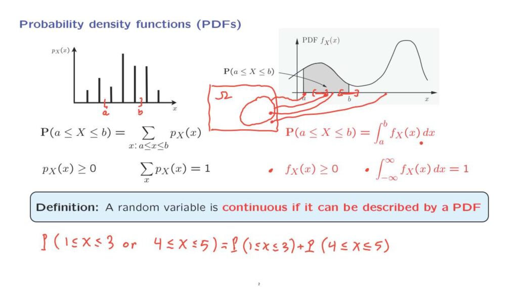
So for example, if we’re looking at the interval from a to b, the probability of this interval is equal to the sum of the probabilities of these three masses that fall inside this interval.
On the other hand, a continuous random variable will be taking values over a continuous range– for example, the real line or an interval on the real line.
Continuous random variables In this case, we still have one total unit of probability mass that is assigned to the possible values of the random variable, except that this unit of mass is spread all over the real line.
But it is not spread in a uniform manner.
Some parts of the real line have more mass per unit length.
Some have less.
How much mass exactly is sitting on top of each part of the real line is described by the probability density function, this function plotted here, which we denote with this notation.
The letter f will always indicate that we are dealing with a PDF.
And the subscript will indicate which random variable we’re talking about.
We use the probability density function to calculate the probability that X lies in a certain interval– let’s say the interval from a to b.
And we calculate it by finding the area under the PDF that sits on top of that interval.
So this area here, the shaded area, is the probability that X stakes values in this interval.
Think of probability as snow fall.
There is one pound of snow that has fallen on top of the real line.
The PDF tells us the height of the snow accumulated over a particular point.
We then find the weight of the overall amount of snow sitting on top of an interval by calculating the area under this curve.
Of course, mathematically, area under the curve is just an integral.
So the probability that X takes values in this interval is the integral of the PDF over this particular interval.
What properties should the PDF have? By analogy with the discrete case, a PDF must be non-negative, because we do not want to get negative probabilities.
In the discrete case, the sum of the PMF entries has to be equal to 1.
In the continuous case, X is certain to lie in the interval between minus infinity and plus infinity.
So letting a be minus infinity and b plus infinity, we should get a probability of 1.
So the total area under the PDF, when we integrate over the entire real line, should be equal to 1.
These two conditions are all that we need in order to have a legitimate PDF.
We can now give a formal definition of what a continuous random variable is.
A continuous random variable is a random variable whose probabilities can be described by a PDF according to a formula of this type.
An important point– the fact that a random variable takes values on a continuous set is not enough to make it what we call a continuous random variable.
For a continuous random variable, we’re asking for a bit more– that it can be described by a PDF, that a formula of this type is valid.
Now, once we have the probabilities of intervals as given by a PDF, we can use of additivity to calculate the probabilities of more complicated sets.
For example, if you’re interested in the probability that X lies between 1 and 3 or that X lies between 4 and 5– so this is the probability that X falls in a region that consists of two disjoint intervals.
We find the probability of the union of these two intervals, by additivity, by adding the probabilities of the two intervals, since these intervals are disjoint.
And then we can use the PDF to calculate the probabilities of each one of these intervals according to this formula.
At this point, you may be wondering what happened to the sample space in all this discussion.
Well, there is still an underlying sample space lurking in the background.
And different outcomes in the sample space result in different numerical values for the random variable of interest.
And when we talk about the probability that X takes values between some numbers a and b, what we really mean is the probability of those outcomes for which the resulting value of X lies inside this particular interval.
So that’s what probability means.
On the other hand, once we have a PDF in our hands, we can completely forget about the underlying sample space.
And we can carry out any calculations we may be interested in by just working with the PDF.
So as we move on in this course, the sample space will be moved offstage.
There will be less and less mention of it.
And we will be working just directly with PDFs or with PMFs if we are dealing with discrete random variables.
Probability of small intervals Let us now build a little bit on our understanding of what PDFs really are by looking at probabilities of small intervals.
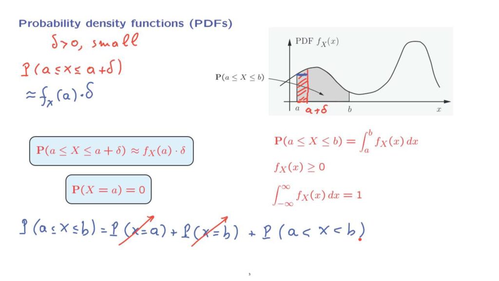
Let us look at an interval that starts at some a and goes up to some number a plus delta.
So here, delta is a positive number.
But we’re interested in the case where delta is very small.
Let us look at the probability that X falls in this interval.
The probability that X lies inside this interval is the area of this region.
On the other hand, as long as f does not change too much over this little interval, which will be the case if we have a continuous density f, then we can approximate the area we have of this region by the area of a rectangle where we keep the height constant.
The area of this rectangle is equal to the height, which is the value of the PDF at the point a, times the base of the rectangle, which is equal to delta.
So this gives us an interpretation of PDFs in terms of probabilities of small intervals.
If we take this factor of delta and send it to the other side in this approximate equality, we see that the value of the PDF can be interpreted as probability per unit length.
So PDFs are not probabilities.
They are densities.
Their units are probability per unit length.
Now, if the probability per unit length is finite and the length delta is sent to 0, we will get 0 probability.
More formally, if we look at this integral and we let b to be the same as a, then we obtain the probability that X is equal to a.
And on that side, we get an integral over a 0 length interval.
And that integral is going to be 0.
So we obtain that the probability that X takes a value equal to a specific, particular point– that probability is going to be equal to 0.
So for a continuous random variable, any particular point has 0 probability.
Yet somehow, collectively, the infinitely many points in an interval together will have positive probablility.
Is this a puzzle? Not really.
That’s exactly what happens, also, with the ordinary notion of length.
Single points have 0 length, yet by putting together lots of points, we can create a set that has a positive length.
And a final consequence of the fact that individual points have 0 length.
Using the additivity axiom, the probability that our random variable takes values inside an interval is equal to the probability that our random variable takes a value of a plus the probability that our random variable takes a value of b plus the probability that our random variable is strictly between a and b.
According to our discussion, this term is equal to 0.
And this term is equal to 0.
And so we conclude that the probability of a closed interval is the same as the probability of an open interval.
When calculating probabilities, it does not matter whether we include the endpoints or not.