In this segment, we will derive the formula for the variance of the geometric PMF.
The argument will be very much similar to the argument that we used to drive the expected value of the geometric PMF.
And it relies on the memorylessness properties of geometric random variables.
So let X be a geometric random variable with some parameter p.
The way to think about X is like the number of coin flips that it takes until we obtain heads for the first time, where p is the probability of heads at each toss.
Recall now the memorylessness property.
If I tell you that X is bigger than 1– which means that the first trial was a failure— we obtained tails.
Given that event, the remaining number of tosses has the same geometric PMF as if we were just starting at this time.
So it has the same geometric PMF as the unconditional PMF of X.
And this is the property that we exploited in order to find the expected value of X.
Now let us take this observation and add one to the random variables involved and turn this statement to the following version.
The conditional PMF of X– which is this random variable plus 1– is the same as the unconditional PMF of this random variable plus 1.
So it’s the same statement as before except that we added 1.
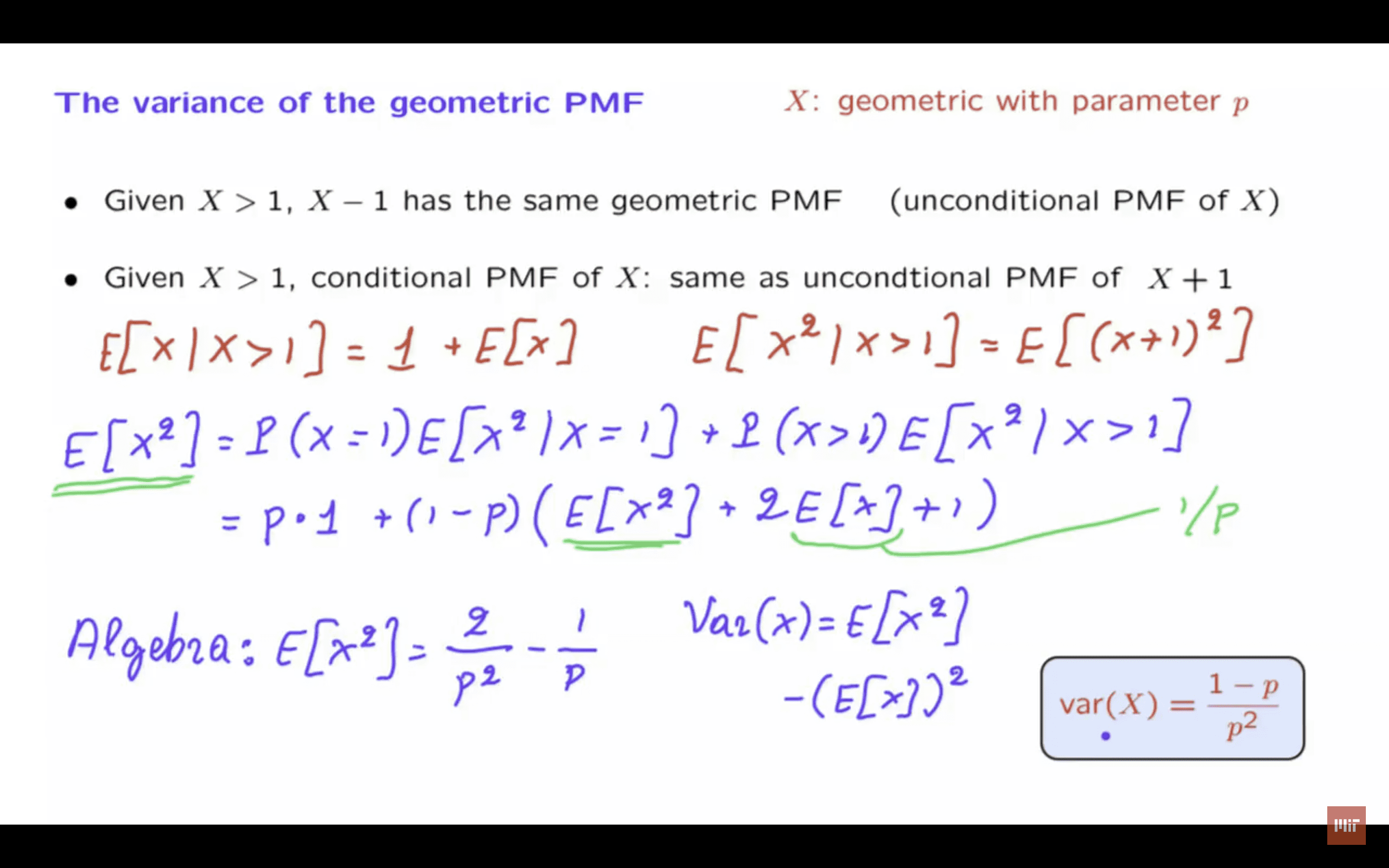
One consequence of the memorylessness that we have already seen and exploited is that the expected value of X in the conditional universe where the first coin flip was wasted is equal to 1– that’s the wasted coin flip– plus how long you expect to have to flip the coin until you obtain heads for the first time, starting from the second flip.
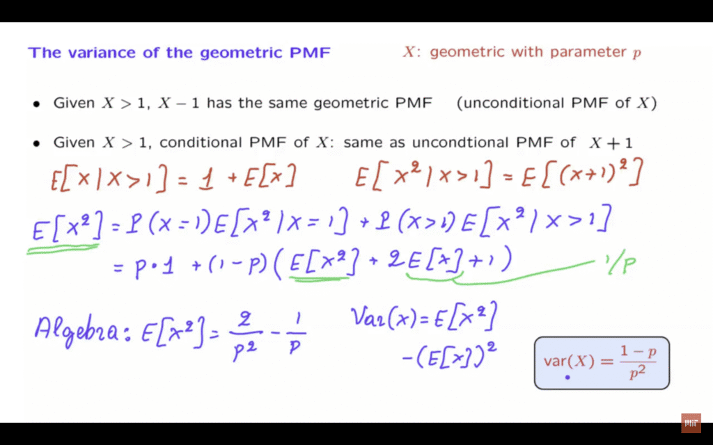
Since the conditional distribution of X in this universe is the same as the unconditional distribution of this random variable, it means that the corresponding expected value in this universe is going to be equal to the expected value of this random variable, which is 1 plus the expected value of X.
And by exactly the same argument, the random variable X squared has the same distribution in the conditional universe as the random variable X plus 1 squared in the unconditional universe.
So since X in the conditional universe has the same distribution as X plus 1, it means that X squared in the conditional universe has the same distribution as X plus 1 squared in the unconditional universe.
So now let us take those facts and use a divide and conquer method to calculate the expected value of X squared.
We will use exactly the same method that we used in order to calculate the expected value.
We separate into two scenarios.
In one scenario, X is equal to 1.
And then we have the expected value of X squared given that X is equal to 1.
And then we have another scenario– the scenario that X is bigger than 1.
And then we have the expected value of X squared given that X is bigger than 1.
So this is just the total expectation theorem.
Now let us calculate terms.
The probability that the first toss results in success, that X is equal to 1– this is p.
And if X is equal to 1, then the value of X squared is also equal to 1.
And then there is probability 1 minus p that the first trial was not a success.
So we get to continue.
We have this conditional expectation here.
But it is equal to this unconditional expectation up there.
And now let us expand the terms in this quadratic and write this as expected value of X squared plus twice the expected value of X plus 1.
Now we know what this expected value here is.
The expected value of a geometric is just 1/p.
And what we’re left with is an equation that involves a single unknown.
Namely, this quantity is the unknown.
And we can solve this linear equation for this unknown.
We carry out some algebra, which is not so interesting by itself.
And after we carry out the algebra, what we obtain is that the expected value of X squared is equal to 2 over p squared minus 1 over p.
And then we use the formula that the variance of a random variable is equal to the expected value of the square of that random variable minus the square of the expected value.
We already know what that expected value is.
We found the expected value of the square.
And putting all that together, we obtain a final answer.
And this is the expression for the variance of a geometric random variable.
It goes without saying that for this calculation to make sense, we need to assume that the parameter that we’re dealing with is positive.