Let us now revisit the variance and see what happens in the case of independence.
Variances have some general properties that we have already seen.
However, since we often add random variables, we would like to be able to say something about the variance of the sum of two random variables.
Unfortunately, the situation is not so simple, and in general, the variance of the sum is not the same as the sum of the variances.
We will see an example shortly.
On the other hand, when X and Y are independent, the variance of the sum is equal to the sum of the variances, and this is a very useful fact.
Let us go through the derivation of this property.
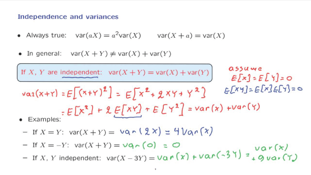
But to keep things simple, let us assume just for the sake of the derivation, that the two random variables have 0 mean.
So in that case, the variance over the sum is just the expected value of the square of the sum.
And we can expand the quadratic and write this as the expectation of X squared plus 2 X Y plus Y squared.
Then we use linearity of expectations to write this as the expected value of X squared plus twice the expected value of X times Y and then plus the expected value of Y squared.
Now, the first term is just the variance of X because we have assumed that we have 0 mean.
The last term is similarly the variance of Y.
How about the middle term? Because of independence, the expected value of the product is the same as the product of the expected values, and the expected values are 0 in our case.
So this term, because of independence, is going to be equal to 0.
In particular, what we have is that the expected value of XY equals the expected value of X times the expected value of Y, equal to 0.
And so we have verified that indeed the variance of the sum is equal to the sum of the variances.
Let us now look at some examples.
Suppose that X is the same random variable as Y.
Clearly, this is a case where independence fails to hold.
If I tell you the value of X, then you know the value of Y.
So in this case, the variance of the sum is the same as the variance of twice X.
Since X is the same as Y, X plus Y is 2 times X.
And then using this property for the variance, what happens when we multiply by a constant? This is going to be 4 times the variance of X.
In another example, suppose that X is the negative of Y.
In that case, X plus Y is identically equal to 0.
So we’re dealing with a random variable that takes a constant value.
In particular, it is always equal to its mean, and so the difference from the mean is always equal to 0, and so the variance will also evaluate to 0.
So we see that the variance of the sum can take quite different values depending on the sort of interrelation that we have between the two random variables.
So these two examples indicate that knowing the variance of each one of the random variables is not enough to say much about the variance of the sum.
The answer will generally depend on how the two random variables are related to each other and what kind of dependencies they have.
As a last example, suppose now that X and Y are independent.
X is independent from Y, and therefore X is also independent from minus 3Y.
Therefore, this variance is equal to the sum of the variances of X and of minus 3Y.
And using the facts that we already know, this is going to be equal to the variance of X plus 9 times the variance of Y.
As an illustration of the usefulness of the property of the variance that we have just established, we will now use it to calculate the variance of a binomial random variable.
Remember that a binomial with parameters n and p corresponds to the number of successes in n independent trials.
We use indicator variables.
This is the same trick that we used to calculate the expected value of the binomial.
So the random variable X sub i is equal to 1 if the i-th trial is a success and is a 0 otherwise.
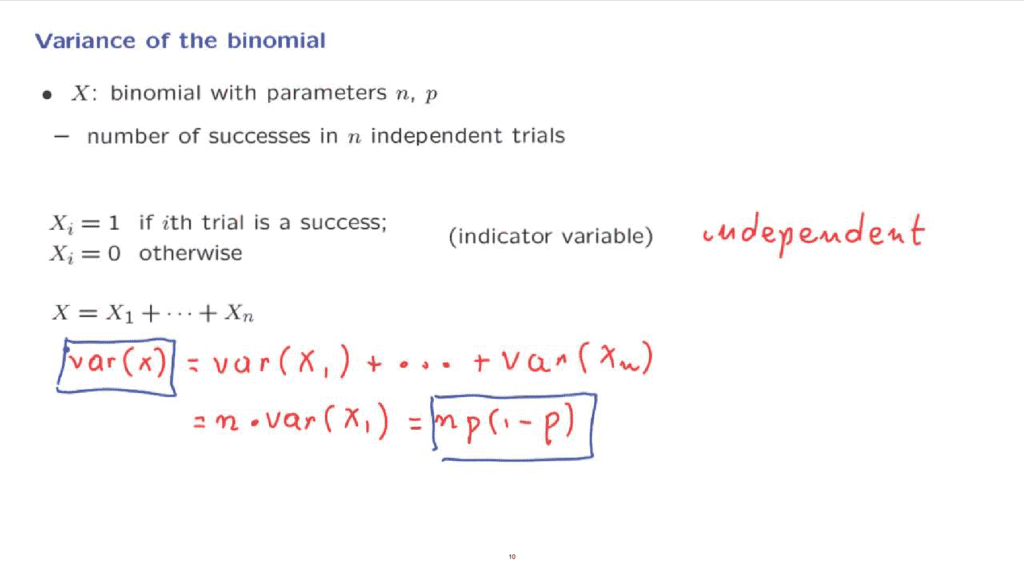
And as we did before, we note that X, the total number of successes, is the sum of those indicator variables.
Each success makes one of those variables equal to 1, so by adding those indicator variables, we’re just counting the number of successes.
The key point to note is that the assumption of independence that we’re making is essentially the assumption that these random variables Xi are independent of each other.
So we’re dealing with a situation where we have a sum of independent random variables, and according to what we have shown, the variance of X is going to be the sum of the variances of the Xi’s.
Now, the Xi’s all have the same distribution so all these variances will be the same.
It suffices to consider one of them.
Now, X1 is a Bernoulli random variable with parameter p.
We know what its variance is– it is p times 1 minus p.
And therefore, this is the formula for the variance of a binomial random variable.