We will now talk about conditional expectations of one random variable given another.
As we will see, there will be nothing new here, except for older results but given in new notation.
Any PMF has an associated expectation.
And so conditional PMFs also have associated expectations, which we call conditional expectations.
We have already seen them for the case where we condition on an event, A.
The case where we condition on random variables is exactly the same.
We let the event, A, be the event that Y takes on a specific value.
And then we calculate the expectation using the relevant conditional probabilities, those that are given by the conditional PMF.
So the conditional expectation of X given that Y takes on a certain value is defined as the usual expectation, except that we use the conditional probabilities that apply given that Y takes on a specific value little y.
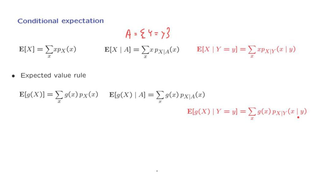
Recall now the expected value rule for ordinary expectations.
And also the Expected Value Rule for conditional expectations given an event, something that we have already seen.
Now, in PMF notation, the expected value rule takes a similar form.
The event, A is replaced by the specific event that Y takes on a specific value.
And in that case, the conditional PMF given the event A is just the conditional PMF given that random variable Y takes on a specific value, little y.
For the case where we condition on events, we also developed a version of the total probability theorem and the total expectation theorem.
We can do the same when we condition on random variables.
So suppose that the sample space has been partitioned into n, disjoint scenarios.
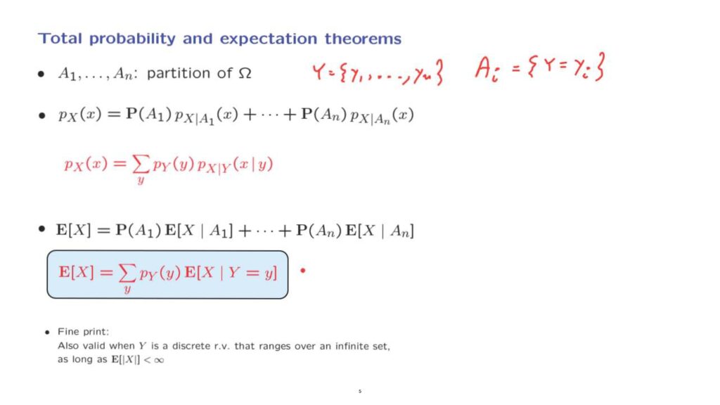
The total probability theorem tells us that the probability of the event that random variable X takes on a value little x, can be found by taking the probabilities of this event under each one of the possible scenarios.
And then weighing those probabilities according to the probabilities of the different scenarios.
Now, suppose that we are dealing with a random variable that takes values in a set consisting of n elements.
And let us consider scenarios Ai, the i-th scenario is the event that the random variable Y takes on the i-th possible value.
We can apply the total probability theorem to this situation.
We can find the probability that the random variable X takes on a certain value, little x, by considering the probability of this event happening under each possible scenario, where a scenario is that Y took on a specific value, and then weigh those probabilities according to the probabilities of the different scenarios.
The story with the total expectation theorem is similar.
We know that an expectation can be found by taking the conditional expectations under each one of the scenarios and weighing them according to the probabilities of the different scenarios.
Again, let the event that Y takes on a specific value be a different scenario.
And with this correspondence we obtain the following version of the total expectation theorem.
We have a sum of different terms.
And each term in the sum is the probability of a given scenario times the expected value of X under this particular scenario.
At this point, I have to add a comment of a more mathematical flavor.
We have been talking about a partition of the sample space into finitely many scenarios.
But if Y takes on values in a discrete but infinite set, for example, if Y can take on any integer value, the argument that we have given is not quite complete.
Fortunately, the total probability theorem and the total expectation theorem, they both remain true, even for the case where Y ranges over an infinite set as long as the random variable X has a well-defined expectation.
For the total probability theorem, the proof for the general case can be carried out without a lot of difficulty, just using the countable additivity axiom.
However, for the total expectation theorem, it takes some harder mathematical work.
And this is beyond our scope.
But we will just take this fact for granted, that the total expectation theorem carries over to the case where we’re adding over an infinite sequence of possible values of Y.
In the rest of the course we will often use the total expectation theorem, including in cases where Y ranges over an infinite discrete set.
In fact, we will see that this theorem is an extremely useful tool that can be used to divide and conquer complicated models.