By this point, we have discussed pretty much everything that is to be said about individual discrete random variables.
Now let us move to the case where we’re dealing with multiple discrete random variables simultaneously, and talk about their distribution.
As we will see, their distribution is characterized by a so-called joint PMF.
So suppose that we have a probabilistic model, and on that model we have defined two random variables– X and Y.
And that we have available their individual PMFs.
These PMFs tell us about one random variable at the time.
This tells us about X, this tells us about Y.
But they do not give us any information about how the two random variables are related to each other.
For example, if you wish to answer this question, whether the numerical values that the two random variables happen to be equal, and what is the probability of that event, you will not be able to answer this question if you only know the two individual PMFs.
In order to be able to answer a question of this type, we will need information that tells us what values of X tend to occur together with what values of Y.
And this information is captured in the so-called joint PMF.
So the joint PMF is nothing but a piece of notation for an object that’s familiar.
This is the probability that when we carry out the experiment we happen to see random variable X take on a value, little x.
And simultaneously see that random variable Y takes on a value, little y.
This quantity we indicate it with this notation.
The letter little p stands for a PMF.
The subscripts tell us which random variables we’re talking about.
And finally, this is a function of two arguments.
Depending on what pair (x,y) we’re interested in, we’re going to get a different numerical value for this probability.
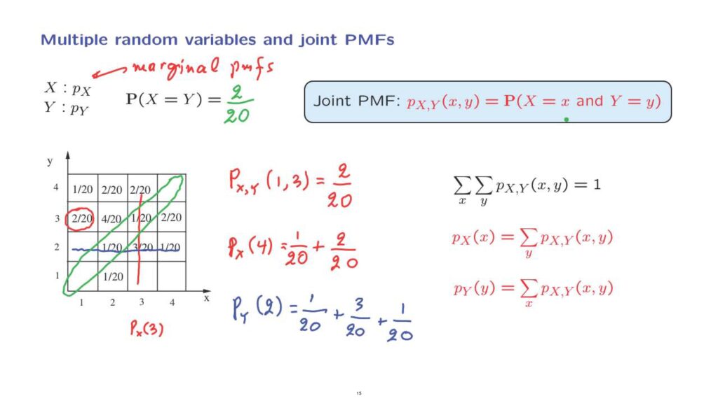
As an example of a joint PMF in which the two random variables take values in a finite set, we might be given a table of this form.
Using this table, we can answer questions such as the following– what is the probability that the random variables X and Y simultaneously take the values, let us say, 1 and 3? Then we look up in this table, and we identify that it’s this probability, X takes the value of 1, and Y takes the value of 3.
And according to this table, the answer would be 2/20.
Now, something to notice about joint PMFs.
When you add over all possible pairs, x and y, this exhausts all the possibilities.
And therefore, these probabilities should add to 1.
In terms of this table, all of the entries that we have here should add to 1.
Now, once we have in our hands the joint PMF, we can use it to find the individual PMFs of the random variables X and Y.
And these individual PMFs are called the marginal PMFs.
How do we find them? Well, the joint PMF tells us everything there is to be known about the two random variables, so it should contain enough information for us to answer any kind of question.
So for example, if we wish to find the probability that the random variable X takes the value of 4, we look at all possible outcomes in which X is equal to 4, and add the probabilities of these outcomes.
So in this case, it would be 1/20 plus 2/20.
So what we’re doing is that if we’re interested in a specific value of X, the probability that X takes on a specific value, we consider all possible pairs associated with that fixed x.
That is, we’re considering one column of the PMF, and we’re adding the corresponding probabilities.
So to find this entry here, let’s say px(3), what we need is to add these terms on that column.
Similarly, we can find the PMF of the random variable Y.
So for example, the probability that the random variable Y takes on a value of, let’s say, 2, can be found as follows.
You look at the probabilities of all pairs associated with this specific y, and you add over the x’s.
So we fix Y to have a value of 2, and we add over all pairs in this row.
So in this example, it would be 1/20 plus 3/20, plus 1/20.
Finally, notice that we are able to answer the question that got us motivated in the first place.
To find the probability that the two random variables take equal values, we look at all the outcomes for which the two random variables indeed take the same numerical values.
And we see that it is this event in this diagram, and the probability of that event is going to be 2/20.
So in general, once we have available the joint PMF of two random variables, we will be able to answer any questions regarding probabilities of events that have to do with these two random variables.
How about more than two random variables? It’s just a matter of notation.
For example, we can define the joint PMF of three random variables, and you can use the same idea for the joint PMF, let’s say, of five, or 10, or n random variables.
Let’s just look at the notation for three.
There is a well-defined probability that when we carry out the experiment X, Y and Z as random variables take on certain specific values.
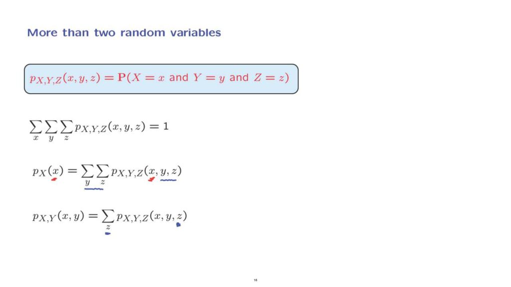
So we look at the probability of that particular triple, and we indicate that probability with this notation.
Once more, the sub-scripts tell us which random variables we’re talking about.
And the PMF, of course, is going to be a function of this triple, little x, little y, little z, because each triple in general should have a different probability.
Of course, probabilities must always add to 1.
So when we consider all triples and we add their corresponding probabilities, we should get 1.
And finally, once we have the joint PMF, we can again recover the marginal PMF.
For example, to find the probability that the random variable takes on a specific value, little x, we consider all possible triples in which the random variable indeed takes that value, little x.
And then we sum over all the possible y’s and z’s that could go together with this particular x.
In the same spirit, to find the probability that these two random variables take on two specific values, we consider all the possible z’s that could go together with this (x,y) pair.
So this way we’re ranging over all outcomes in which X and Y take on these specific values.
But Z is free to take any value, and so we consider all those possible values of Z and sum the corresponding probabilities.
Finally, we can talk about functions of multiple random variables.
Suppose that we have two random variables, x and y, and that we define a function of them.
So this function is, of course, a random variable.
And we can find the PMF of this random variable if we know the joint PMF of X and Y.
So the PMF, which is the probability that the random variable takes on a specific numerical value, that’s the probability that the function of X and Y takes on a specific numerical value.
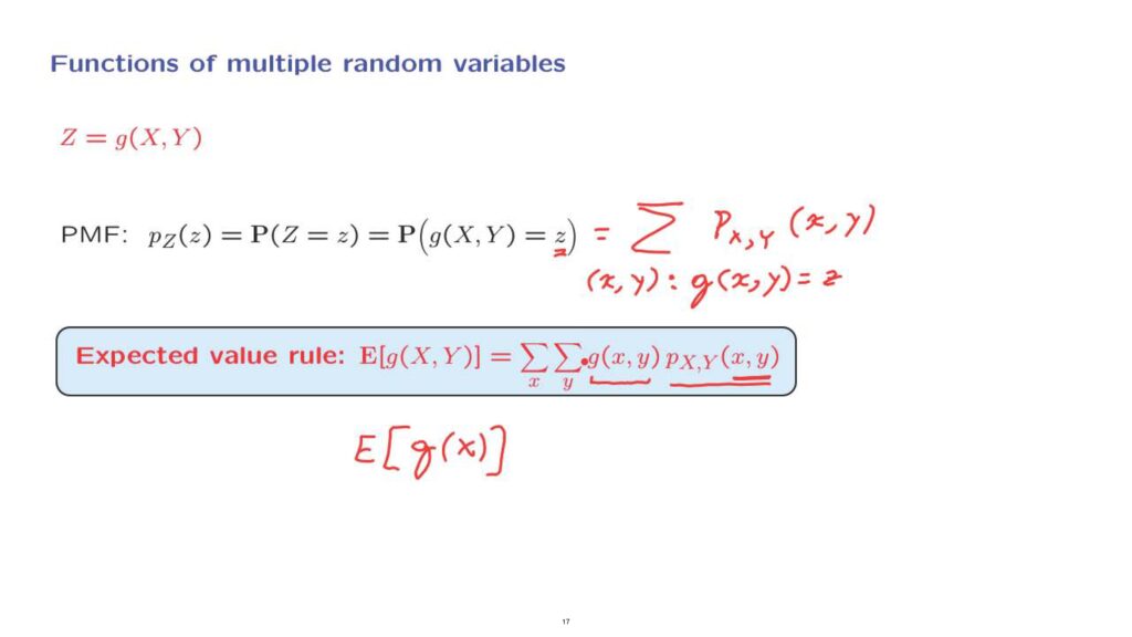
And we can find this probability by adding the probabilities of all (x,y) pairs.
Which (x,y) pairs? Those (x,y) pairs for which the value of Z would be equal to this particular number, little z, that we care about.
So we collect essentially all possible outcomes that make this event to happen, and we add the probabilities of all those outcomes.
Finally, similarly to the case where we have a single random variable and function of it, we now can talk about expected values of functions of two random variables, and there is an expected value rule that parallels the expected value rule that we had developed for the case of a function of this form.
The form that the expected value rule takes is similar, and it’s quite natural.
The interpretation is as follows.
With this probability, a specific (x,y) pair will occur.
And when that occurs, the value of our random variable is a certain number.
And the combination of these two terms gives us a contribution to the expected value.
Now, we consider all possible (x,y) pairs that may occur, and we sum over all these (x,y) pairs.