In this segment, we will go through the calculation of the variances of some familiar random variables, starting with the simplest one that we know, which is the Bernoulli random variable.
So let X take values 0 or 1, and it takes a value of 1 with probability p.
We have already calculated the expected value of X, and we know that it is equal to p.
Let us now compute its variance.
One way of proceeding is to use the definition and then the expected value rule.
So if we now apply the expected value rule, we need the summation over all possible values of X.
There are two values– x equal to 1 or x equal to 0.
The contribution when X is equal to 1 is 1 minus the expected value, which is p squared.
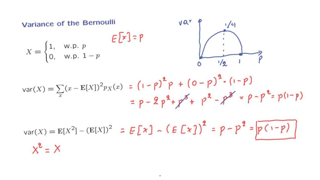
And the value of 1 is taken with probability p.
There is another contribution to this sum when little x is equal to 0.
And that contribution is going to be 0 minus p, all of this squared, times the probability of 0, which is 1 minus p.
And now we carry out some algebra.
We expand the square here, 1 minus 2p plus p squared.
And after we multiply with this factor of p, we obtain p minus 2p squared plus p to the third power.
And then from here we have a factor of p squared times 1, p squared times minus p.
That gives us a minus p cubed.
Then we notice that this term cancels out with that term.
p squared minus 2p squared leaves us with p minus p squared.
And we factor this as p times 1 minus p.
An alternative calculation uses the formula that we provided a little earlier.
Let’s see how this will go.
We have the following observation.
The random variable X squared and the random variable X– they are one and the same.
When X is 0, X squared is also 0.
When X is 1, X squared is also 1.
So as random variables, these two random variables are equal in the case where X is a Bernoulli.
So what we have here is just the expected value of X minus the expected value of X squared, to the second power.
And this is p minus p squared, which is the same answer as we got before– p times 1 minus p.
And we see that the calculations and the algebra involved using this formula were a little simpler than they were before.
Now the form of the variance of the Bernoulli random variable has an interesting dependence on p.
It’s instructive to plot it as a function of p.
So this is a plot of the variance of the Bernoulli as a function of p, as p ranges between 0 and 1.
p times 1 minus p is a parabola.
And it’s a parabola that is 0 when p is either 0 or 1.
And it has this particular shape, and the peak of this parabola occurs when p is equal to 1/2, in which case the variance is 1/4.
In some sense, the variance is a measure of the amount of uncertainty in a random variable, a measure of the amount of randomness.
A coin is most random if it is fair, that is, when p is equal to 1/2.
And in this case, the variance confirms this intuition.
The variance of a coin flip is biggest if that coin is fair.
On the other hand, in the extreme cases where p equals 0– so the coin always results in tails, or if p equals to 1 so that the coin always results in heads– in those cases, we do not have any randomness.
And the variance, correspondingly, is equal to 0.
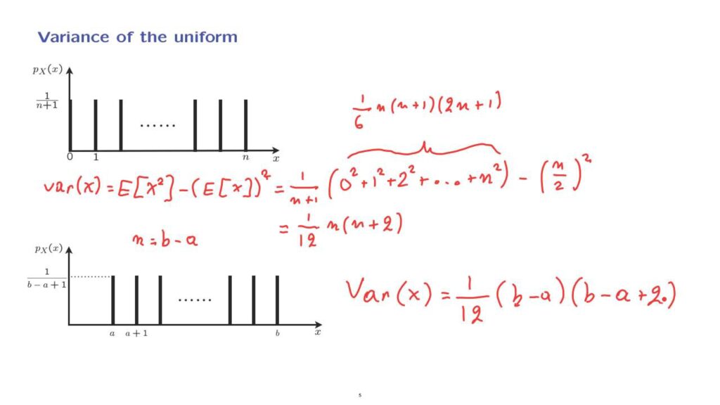
Let us now calculate the variance of a uniform random variable.
Let us start with a simple case where the range of the uniform random variable starts at 0 and extends up to some n.
So there is a total of n plus 1 possible values, each one of them having the same probability– 1 over n plus 1.
We calculate the variance using the alternative formula.
And let us start with the first term.
What is it? We use the expected value rule, and we argue that with probability 1 over n plus 1, the random variable X squared takes the value 0 squared, with the same probability, takes the value 1 squared.
With the same probability, it takes the value 2 squared, and so on, all of the way up to n squared.
And then there’s the next term.
The expected value of the uniform is the midpoint of the distribution by symmetry.
So it’s n over 2, and we take the square of that.
Now to make progress here, we need to evaluate this sum.
Fortunately, this has been done by others.
And it turns out to be equal to 1 over 6 n, n plus 1 times 2n plus 1.
This formula can be proved by induction, but we will just take it for granted.
Using this formula, and after a little bit of simple algebra and after we simplify, we obtain a final answer, which is of the form 1 over 12 n times n plus 2.
How about the variance of a more general uniform random variable? So suppose we have a uniform random variable whose range is from a to b.
How is this PMF related to the one that we already studied? First, let us assume that n is chosen so that it is equal to b minus a.
So in that case, the difference between the last and the first value of the random variable is the same as the difference between the last and the first possible value in this PMF.
So both PMFs have the same number of terms.
They have exactly the same shape.
The only difference is that the second PMF is shifted away from 0, and it starts at a instead of starting at 0.
Now what does shifting a PMF correspond to? It essentially amounts to taking a random variable– let’s say, with this PMF– and adding a constant to that random variable.
So if the original random variable takes the value of 0, the new random variable takes the value of a.
If the original takes the value of 1, this new random variable takes the value of a plus 1, and so on.
So this shifted PMF is the PMF associated to a random variable equal to the original random variable plus a constant.
But we know that adding a constant does not change the variance.
Therefore, the variance of this PMF is going to be the same as the variance of the original PMF, as long as we make the correspondence that n is equal to b minus a.
So doing this substitution in the formula that we derived earlier, we obtain 1 over 12 b minus a times b minus a plus 2.