Our discussion of random variable so far has involved nothing but standard probability calculations.
Other than using the PMF notation, we have done nothing new.
It is now time to introduce a truly new concept that plays a central role in probability theory.
This is the concept of the expected value or expectation or mean of a random variable.
It is a single number that provides some kind of summary of a random variable by telling us what it is on the average.
Let us motivate with an example.
You play a game of chance over and over, let us say 1,000 times.
Each time that you play, you win an amount of money, which is a random variable, and that random variable takes the value 1, with probability 2/10, the value of 2, with probability 5/10, the value of 4, with probability 3/10.
You can plot the PMF of this random variable.
It takes values 1, 2, and 4.
And the associated probabilities are 2/10, 5/10, and 3/10.
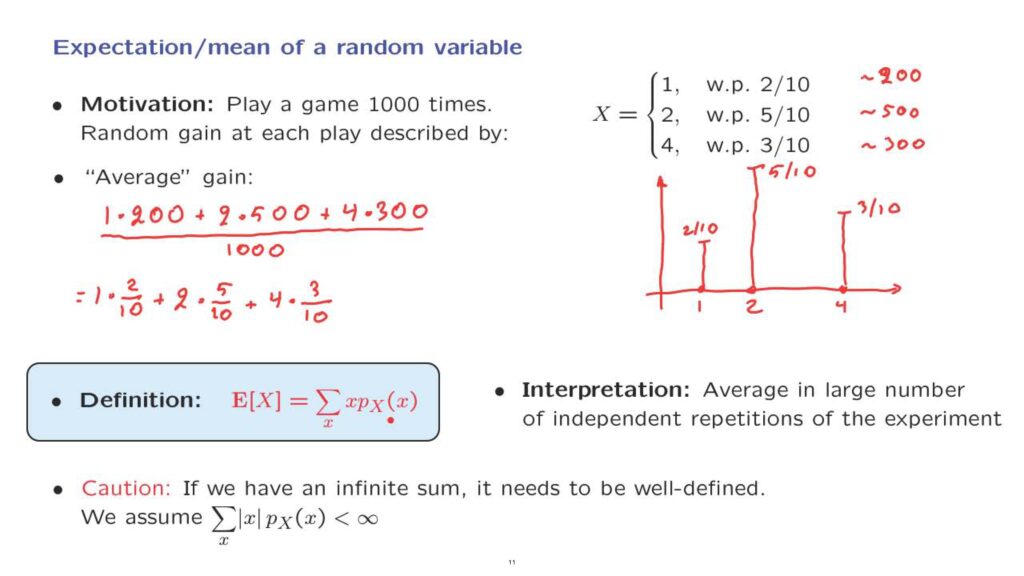
How much do you expect to have at the end of the day? Well, if you interpret probabilities as frequencies, in a thousand plays, you expect to have about 200 times this outcome to occur and this outcome about 500 times and this outcome about 300 times.
So your average gain is expected to be your total gain, which is 1, 200 times, plus 2, 500 times, plus 4, 300 times.
This is your total gain.
And to get to the average gain, you divide by 1,000.
And the expression that you get can also be written in a simpler form as 1 times 2/10 plus 2 times 5/10 plus 4 times 3/10.
So this is what you expect to get, on the average, if you keep playing that game.
What have we done? We have calculated a certain quantity which is a sort of average of the random variable of interest.
And what we did in this summation here, we took each one of the possible values of the random variable.
Each possible value corresponds to one term in the summation.
And what we’re adding is the numerical value of the random variable times the probability that this particular value is obtained.
So when x is equal to 1, we get 1 here and then the probability of 1.
When we add the term corresponding to x equals 2, we get little x equals to 2 and next to it the probability that x is equal to 2, and so on.
So this is what we call the expected value of the random variable x.
This is the formula that defines it, but it’s also important to always keep in mind the interpretation of that formula.
The expected value of a random variable is to be interpreted as the average that you expect to see in a large number of independent repetitions of the experiment.
One small technical caveat, if we’re dealing with a random variable that takes values in a discrete but infinite set, this sum here is going to be an infinite sum or an infinite series.
And there’s always a question whether an infinite series has a well-defined limit or not.
In order for it to have a well-defined limit, we will be making the assumption that this infinite series is, as it’s called, absolutely convergent, namely that if we replace the x’s by their absolute values– so we’re adding positive numbers, or nonnegative numbers– the sum of those numbers is going to be finite.
So this is a technical condition that we need in order to make sure that this expected value is a well-defined and finite quantity.
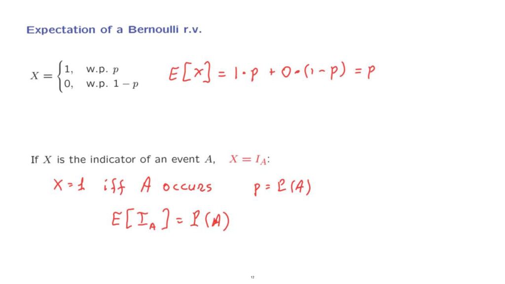
Let us now calculate the expected value of a very simple random variable, the Bernoulli random variable that takes the value 1 with probability p and the value 0 with probability 1 minus p.
The expected value consists of two terms.
X can take the value 1.
This happens with probability p.
Or it can take the value of zero.
This happens with probability 1 minus p.
And therefore, the expected value is just equal to p.
As a special case, we may consider the situation where X is the indicator random variable of a certain event, A, so that X is equal to 1 if and only if event A occurs.
In this case, the probability that X equals to 1, which is our parameter p, is the same as the probability that event A occurs.
And we have this relation.
And so with this correspondence, we readily conclude that the expected value of an indicator random variable is equal to the probability of that event.
Let us move now to the calculation of the expected value of a uniform random variable.
Let us consider, to keep things simple, a random variable which is uniform on the set from 0 to n.
It’s uniform, so the probability of the values that it can take are all equal to each other.
It can take one of n plus 1 possible values, and so the probability of each one of the values is 1 over n plus 1.
We want to calculate the expected value of this random variable.
How do we proceed? We just recall the definition of the expectation.
It’s a sum where we add over all of the possible values.
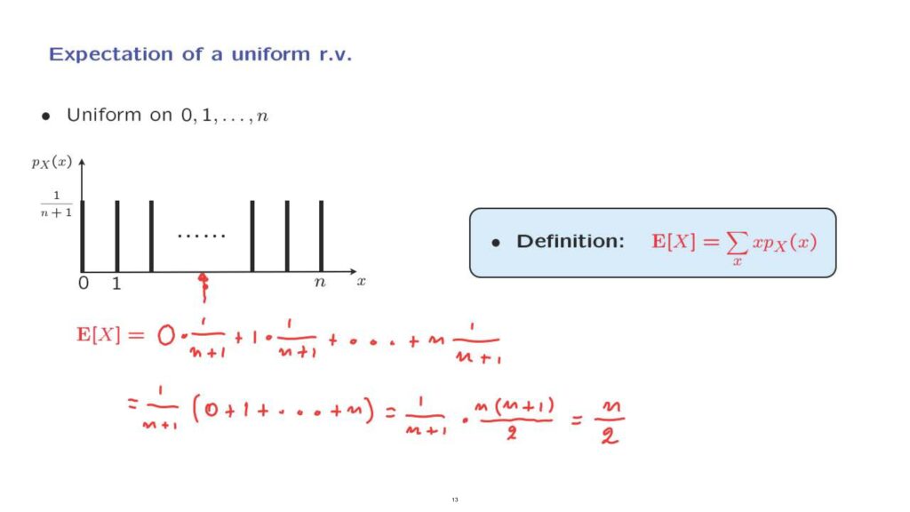
And for each one of the values, we multiply by its corresponding probability.
So we obtain a summation of this form.
We can factor out a factor of 1 over n plus 1, and we’re left with 0 plus 1 plus all the way up to n.
And perhaps you remember the formula for us summing those numbers, and it is n times n plus 1 over 2.
And after doing the cancellations, we obtain a final answer, which is n over 2.
Incidentally, notice that n over 2 is just the midpoint of this picture that we have here in this diagram.
This is always the case.
Whenever we have a PMF which is symmetric around a certain point, then the expected value will be the center of symmetry.
More general, if you do not have symmetry, the expected value turns out to be the center of gravity of the PMF.
If you think of these bars as having weight, where the weight is proportional to their height, the center of gravity is the point at which you should put your finger if you want to balance that diagram so that it doesn’t fall in one direction or the other.
And we now close this segment by providing one more interpretation of expectations.
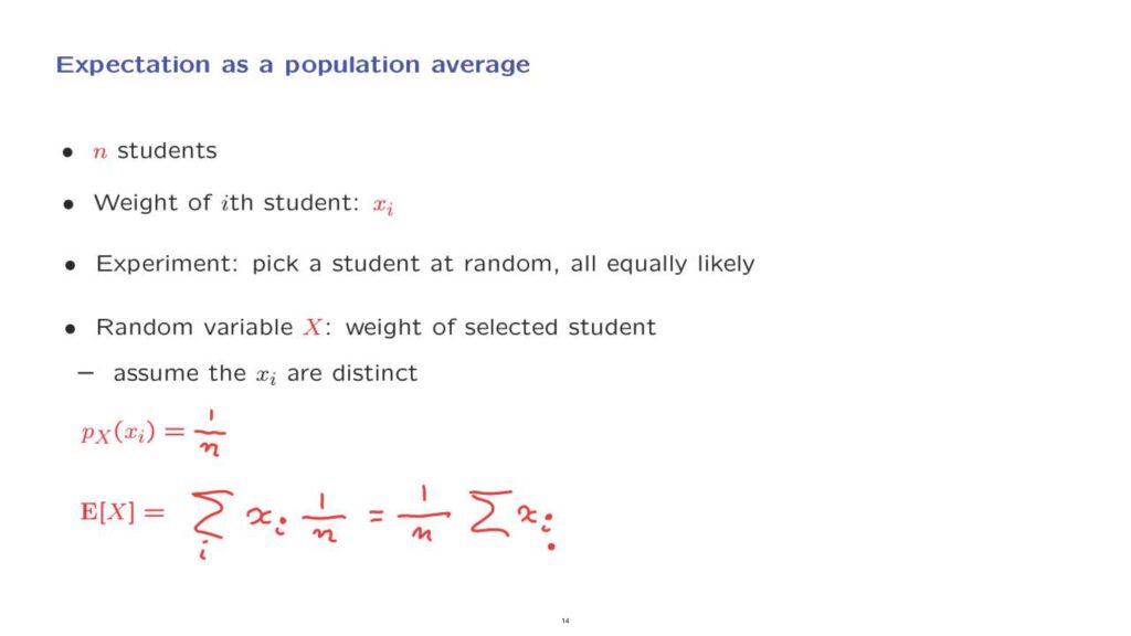
Suppose that we have a class consisting of n students and that the ith student has a weight which is some number xi.
We have a probabilistic experiment where we pick one of the students at random, and each student is equally likely to be picked as any other student.
And we’re interested in the random variable X, which is the weight of the student that was selected.
To keep things simple, we will assume that the xi’s are all distinct.
And we first find the PMF of this random variable.
Any particular xi that this possible is associated to exactly one student, because we assumed that the xi’s are distinct.
So this probability would be the probability or selecting the ith student, and that probability is 1 over n.
And now we can proceed and calculate the expected value of the random variable X.
This random variable X takes values, and the values that it takes are the xi’s.
A particular xi would be associated with a probability 1 over n, and we’re adding over all the i’s or over all of the students.
And so this is the expected value.
What we have here is just the average of the weights of the students in this class.
So the expected value in this particular experiment can be interpreted as the true average over the entire population of the students.
Of course, here we’re talking about two different kinds of averages.
In some sense, we’re thinking of expected values as the average in a large number of repetitions of experiments.
But here we have another interpretation as the average over a particular population.