The last discrete random variable that we will discuss is the so-called geometric random variable.
It shows up in the context of the following experiment.
We have a coin and we toss it infinitely many times and independently.
And at each coin toss we have a fixed probability of heads, which is some given number, p.
This is a parameter that specifies the experiment.
When we say that the infinitely many tosses are independent, what we mean in a mathematical and formal sense is that any finite subset of those tosses are independent of each other.
I’m only making this comment because we introduced a definition of independence of finitely many events, but had never defined the notion of independence or infinitely many events.
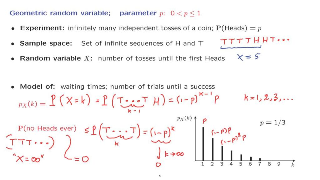
The sample space for this experiment is the set of infinite sequences of heads and tails.

So a typical outcome of this experiment might look like this.
It’s a sequence of heads and tails in some arbitrary order.
And of course, it’s an infinite sequence, so it continues forever.
But I’m only showing you here the beginning of that sequence.
We’re interested in the following random variable, X, which is the number of tosses until the first heads.
So if our sequence looked like this, our random variable would be taking a value of 5.
A random variable of this kind appears in many applications and many real world contexts.
In general, it models situations where we’re waiting for something to happen.
Suppose that we keep doing trials at each time and the trial can result either in success or failure.
And we’re counting the number of trials it takes until a success is observed for the first time.
Now, these trials could be experiments of some kind, could be processes of some kind, or they could be whether a customer shows up in a store in a particular second or not.
So there are many diverse interpretations of the words trial and of the word success that would allow us to apply this particular model to a given situation.
Now, let us move to the calculation of the PMF of this random variable.
By definition, what we need to calculate is the probability that the random variable takes on a particular numerical value.
What does it mean for X to be equal to k? What it means is that the first heads was observed in the k-th trial, which means that the first k minus 1 trials were tails, and then were followed by heads in the k-th trial.

This is an event that only concerns the first k trials, and the probability of this event can be calculated using the fact that different coin tosses or different trials are independent.
It is the probability of tails in the first coin toss times the probability of tails in the second coin toss, and so on, k minus 1 times.
So we get an exponent here of k minus 1 times the probability of heads in the k-th coin toss.
So this is the form of the PMF of this particular random variable, and that formula applies for the possible values of k, which are the positive integers.
Because the time of the first head can only be a positive integer.
And any positive integer is possible, so our random variable takes values in a discrete but infinite set.
The geometric PMF has a shape of this type.
Here we see the plot for the case where p equals to 1/3.
The probability that the first head shows up in the first trial is equal to p, that’s the probability of heads.
The probability that it shows up in the next trial, that the first head appears in the second trial, this is the probability that we had heads following a tail.
So we have the probability of a tail and then times the probability of a head.
And then each time that we move to a further entry, we multiply by a further factor of 1 minus p.
Finally, one little technical remark.
There’s a possible and rather annoying outcome of this experiment, which would be that we observe a sequence of tails forever and no heads.

In that case, our random variable is not well-defined, because there is no first heads to consider.
You might say that in this case our random variable takes a value of infinity, but we would rather not have to deal with random variables that could be infinite.
Fortunately, it turns out that this particular event has 0 probability of occurring, which I will now try to show.
So this is the event that we always see tails.
Let us compare it with the event where we see tails in the first k trials.
How do these two events relate? If we have always tails, then we will have tails in the first k trials.
So this event implies that event.
This event is smaller than that event.
So the probability of this event is less than or equal to the probability of that second event.
And the probability of that second event is 1 minus p to the k.
Now, this is true no matter what k we choose.
And by taking k arbitrarily large, this number here becomes arbitrarily small.
Why does it become arbitrarily small? Well, we’re assuming that p is positive, so 1 minus p is a number less than 1.
And when we multiply a number strictly less than 1 by itself over and over, we get arbitrarily small numbers.
So the probability of never seeing a head is less than or equal to an arbitrarily small positive number.
So the only possibility for this is that it is equal to 0.
So the probability of not ever seeing any heads is equal to 0, and this means that we can ignore this particular outcome.
And as a side consequence of this, the sum of the probabilities of the different possible values of k is going to be equal to 1, because we’re certain that the random variable is going to take a finite value.
And so when we sum probabilities of all the possible finite values, that sum will have to be equal to 1.
And indeed, you can use the formula for the geometric series to verify that, indeed, the sum of these numbers here, when you add over all values of k, is, indeed, equal to 1.