In this segment, we will discuss the multinomial model and the multinomial probabilities, which are a nice generalization of the binomial probabilities.
The setting is as follows.
We are dealing with balls and the balls come into different colors.
There are r possible different colors.
We pick a ball at random, and when we do that, there is a certain probability Pi that the ball that we picked has ith color.
Now, we repeat this process n times independently.
Each time we get a ball that has a random color.
And we’re interested in the following kind of question.
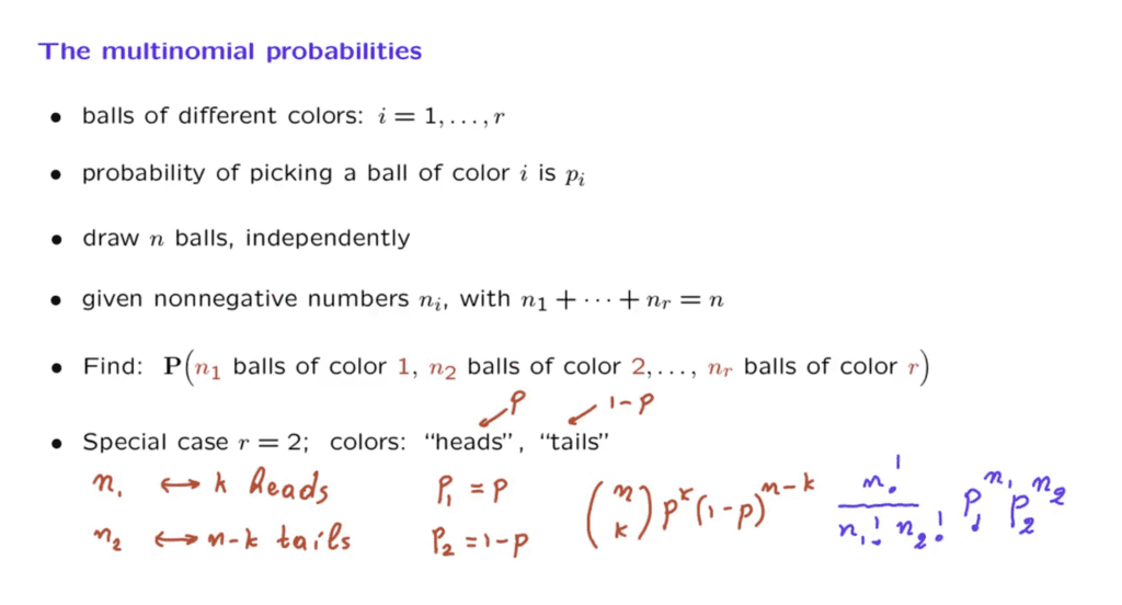
Somebody fixes for us certain numbers– n1, n2, up to nr that add up to n, and asks us, what is the probability that when you carry out the experiment, you get exactly n1 balls of the first color, exactly n2 balls of the second color, and so on? So the numbers n1, n2, up to nr are fixed given numbers.
For a particular choice of those numbers, we want to calculate this probability.
Now of course, this is a more general model.
It doesn’t necessarily deal with balls of different colors.
For example, we might have an experiment that gives us random numbers, where the numbers range from 1 up to r, and at each time we get a random number with probability Pi we get a number which is equal to i.
So we could use this to model die rolls, for example.
And there’s actually a special case of this problem, which should be familiar.
Suppose that we have only two colors, and instead of thinking of colors, let us think of the two possibilities as being heads or tails.
And we can make the following analogy.
Somebody gives us numbers n1 and n2 that add up to n.
And we’re interested in the probability that we get n1 of the first color and n2 of the second color.
Well, we could think of this as a setting in which we are asking for the probability that we obtain k heads and n minus k tails.
So the question of what is the probability that we obtain k heads and n minus k tails is of the same kind as what is the probability that we get n1 of the first color and n2 of the second color.
Now, if heads have a probability p of occurring, and tails has a probability of 1 minus p of occurring, then we would have the following analogy.
The probability of obtaining the first color, which correspond to heads, that would be equal to p.
The probability of obtaining the second color, which correspond to tails, this would be 1 minus p.
Now, the probability of obtaining k heads in those n independent trials– we know what it is.
By the binomial probabilities, it is n choose k times p to the k times one minus p to the power n minus k.
Now we can translate this answer to the multinomial case where we’re dealing with colors, and we do these substitutions.
So n choose k is n factorial divided by k factorial.
In this case, k is the same as n1, so we get n1 factorial.
And then we are going to have here n minus k factorial.
But n minus k corresponds to n2.
So here we get an n2 factorial.
And then p corresponds to p1 and p2 corresponds to 1 minus p.
So we get here p1 times p2.
n to the power n minus k, again, by analogy, is n2.
So this is the form of the multinomial probabilities for the special case where we’re dealing with two colors.
Let us now look at the general case.
Let us start with an example, to be concrete.
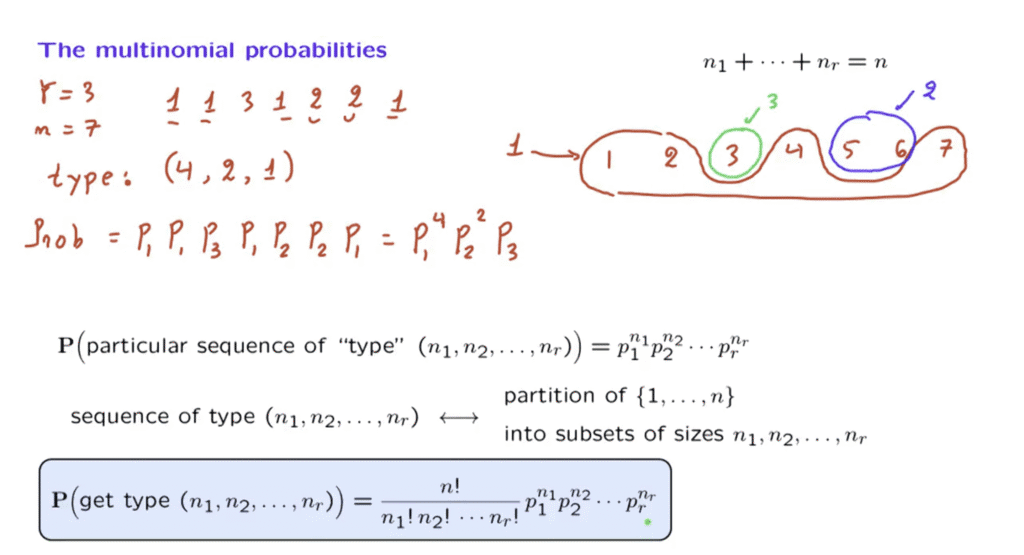
Suppose that the number of colors is equal to 3, and that we’re going to pick n equal to 7 balls.
We carry out the experiments, and we might obtain an outcome which would be a sequence of this type.
So the first ball had the color 1, the second ball had the first color, the third ball had the third color, the fourth ball had the first color, and so on.
And suppose that this was the outcome.
One way of summarizing what happened in this outcome would be to say that we had four 1s, we had two 2s, and we had one 3.
We could say that this is the type of the outcome.
It’s of type 4, 2, 1– that is, we obtained four of the first color, two of the second color, and one of the third color.
This is one possible outcome.
What is the probability of obtaining this particular outcome? The probability of obtaining this particular outcome is, using independence, the probability that we obtain color 1 in the first trial, color 1 in the second trial, color 3 in the third trial, color 1 in the fourth trial, color 2 in the next trial, color 2 in the next trial, color 1 in the last trial.
And we put all the factors together, and we notice that this is p1 to the fourth p2 to the second times p3.
It’s not a coincidence that the exponents that we have up here are exactly the count that we had when we specified the type of this particular outcome.
Generalizing from this example, we realize that the probability of obtaining a particular sequence of a certain type, that probability is of this form.
For each color, we have the probability of that color raised to the power of how many times that particular color appears in a sequence.
So any particular sequence of this type has this probability.
What we’re interested in is to find the total probability of obtaining some sequence of this type.
How can we find this probability? Well, we will take the probability of each sequence of this type– which is this much, and it’s the same for any particular sequence– and multiply with the number of sequences of this type.
So how many sequences are there of a certain type? Let us look back at our example.
We had seven trials.
So let us number here the different trials.
And when I tell you that a particular sequence was obtained, that’s the same as telling you that in this set of trials, we had the first color.
In this set of trials, the fifth and sixth trial, we had the second color.
And in this trial, the third trial, we had the third color.
This is an alternative way of telling you what sequence we obtained.
I tell you at which trials we had the first color, at which trials we had the second, at which trials we had the third.
But What do we have here? Here we have a partition of the set of numbers from 1 up to 7 into three subsets.
And the cardinalities of those subsets are the numbers that appear here in the type of the sequence.
The conclusion is that a sequence of certain type is equivalent, or can be alternatively specified, by giving you a partition over this set of tosses, which is the set from 1 up to n, how many trials we’ve had, a partition into subsets of certain sizes.
So this allows us now to count the number of sequences of a certain type.
It’s exactly the same as the number of partitions, and we know what this is.
And putting everything together, the probability of obtaining a sequence of a certain type is equal to the count of how many sequences do we have of the certain type, which is the same as the number of partitions of a certain type, times the probability of any particular sequence of that type that we’re interested in.
So this is a formula that generalizes the one that we saw before for the case where we have only two colors, and which corresponded to the coin tossing setting.
And it is a useful model, because you can think of many situations in which you have repeated trials, and at each trial, you obtain one out of a finite set of possible results.
There are different possible results.
You repeat those trials independently.
And you may be interested in the question of how many results of the first kind, of the second kind, and so on there will be.