Let us now move from the abstract to the concrete. Recall the example that we discussed earlier where we have two rolls of a tetrahedral die. So there are 16 possible outcomes illustrated in this diagram.
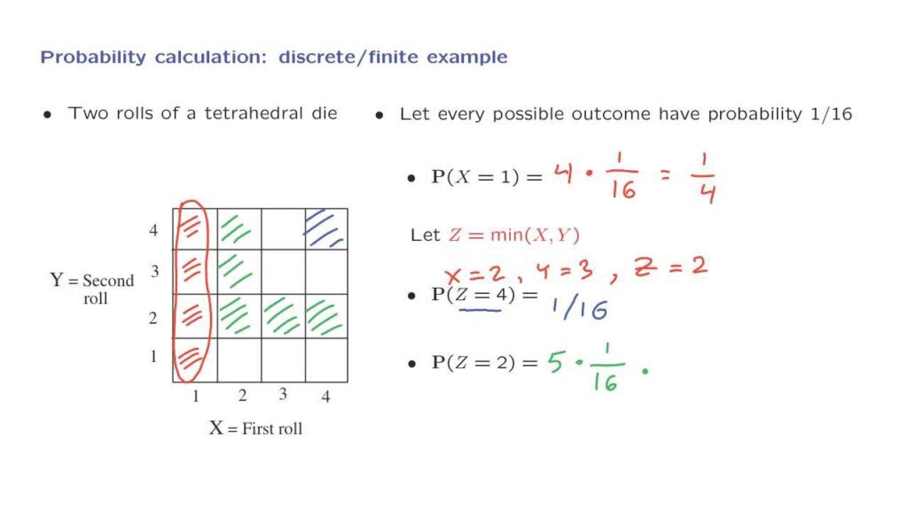
To continue, now we need to specify a probability law, some kind of probability assignment. To keep things simple, we’re going to make the assumption that the 16 possible outcomes are all equally likely. And each outcome has a probability of 1 over 16.
Given this assumption, we will now proceed to calculate certain probabilities. Let us look first at the probability that X, which stands the result of the first roll, is equal to 1.
The way to calculate this probability is to identify what exactly that event is in our picture of the sample space, and then calculate. The event that X is equal to 1 can happen in four different ways that correspond to these four particular outcomes.
Each one of these outcomes has a probability of 1 over 16. The probability of this event is the sum of the probabilities of the outcomes that it contains. So it is 4 times 1 over 16, equal to one fourth. Let now Z stand for the smaller of the two numbers that came up in our two rolls.
So for example, if X is 2 and Y is equal to 3, then Z is equal to 2, which is the smaller of the two. Let us try to calculate the probability that the smaller of the two outcomes is equal to 4.
Now for the smaller of the two outcomes to be equal to 4, we must have that both X and Y are equal to 4. So this outcome here is the only way that this particular event can happen.
Since there’s only one outcome that makes the event happen, the probability of this event is the probability of that outcome and is equal to 1 over 16. For another example, let’s calculate the probability that the minimum is equal to 2.
What does it mean that the minimum is equal to 2? It means that one of the dice resulted in a 2, and the other die resulted in a number that’s 2 or larger. So we could have both equal to 2.
We could have X equal to 2, but Y larger. Or we could have Y equal to 2 and X something larger. This green event, this green set, is the set of all outcomes for which the minimum of the two rolls is equal to 2.
There’s a total of five such outcomes. Each one of them has probably 1 over 16. And we have discussed that for finite sets, the probability of a finite set is the sum of the probabilities of the elements of that set.
So we have five elements here, each one with probability 1 over 16. And this is the answer to this problem.
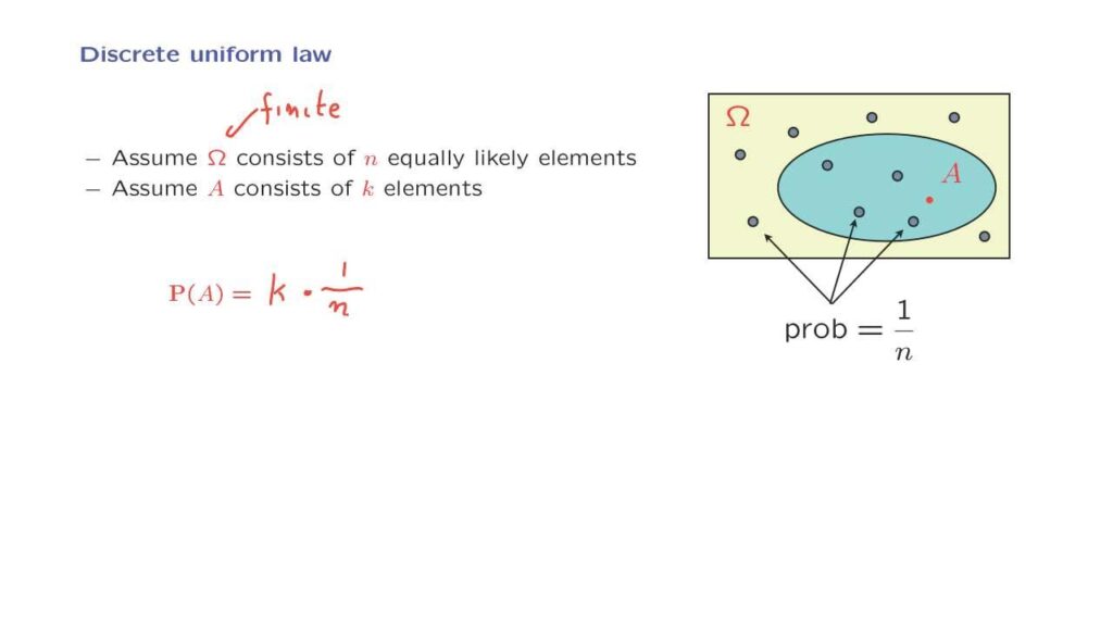
This particular example that we saw here is a special case of what is called a discrete uniform law. In a discrete uniform law, we have a sample space which is finite. And it has n elements. And we assume that these n elements are equally likely. Now since the probability of omega, the probability of the entire sample space, is equal to 1, this means that each one of these elements must have probability 1 over n.
That’s the only way that the sum of the probabilities of the different outcomes would be equal to 1 as required by the normalization axiom. Consider now some subset of the sample space, an event A that, exactly k elements. What is the probability of the set A?
It’s the sum of the probabilities of its elements. There are k elements. And each one of them has a probability of 1 over n. And this way we can find the probability of the set A.
So when we have a discrete uniform probability law, we can calculate probabilities by simply counting the number of elements of omega, which is n, finding the number n, and counting the number of elements of the set A.
That’s the reason why counting will turn out to be an important skill. And there will be a whole lecture devoted to this particular topic.